1. Software for data analysis
Jul 17, 2024·
 ·
6 min read
·
6 min read
Xuefeng Ding
Pre-requisite
You should know
- basic concepts about folders (文件夹) and files (文件),
- simple linux commands such as
cdandls, - and can use some editor such as vim or nano.
Very simple vim tutorial
- There are two mode,
normalandinsert. Watch bottom left. - Press
esc(on top left of your keyboard) toinsert->normal - Press
itonormal->insert - In the
insertmode, you can type. - In the
normalmode- type
:wto save,:w hi.txtto save ashi.txt - type
:qto quit,:wqor:wq hi.txtto save and exit. - type
:q!to quit without saving.
- type
- That’s it. Now you can use
vim.
Get Linux-like shell (Windows)
- If you use windows, it’s better you install WSL.
WSLis like a virtual machine platform like virtualbox or vmware, but designed by microsoft and is more stable and convenient.- With
WSLyou can install a virtual machine with Ubuntu 22.04. We will work in the Ubuntu. - For Mac user, we can just work in the OSX. You can download iTerm2 for better experience compared with the original terminal app.
Install Windows Terminal
Go to Windows store and install the Windows Terminal.
Install WSL
- Follow the Microsoft recipe.
- Open the
Windows Terminaland type
wsl --install
Install Ubuntu 22.04
- Open the
Windows Terminaland type
wsl --status # verify you have WSL 2 installed
wsl --list --online # check available OS to you
wsl --install --d Ubuntu-22.04 # install Ubuntu 22.04
# If it does not work, try wsl --update. You might need a proxy.
- Alternatively, you may also download it from the Windows Store directly.
- If your Windows store is blank, read this article.
Verify installation
- Verify you got
Ubuntu 22.04virtual machine.
wsl -l # verify you have Ubuntu-22.04 listed and marked as default.
wsl --set-default Ubuntu-22.04 # if not default, use this command
- Now you can enter your
Ubuntu 22.04virtual machine by- Open
Windows Terminaland chooseUbuntu 22.04profile - Or Open
Windows Terminaland chooseCommand Promptand type
wsl - Open
Setup package manger
Install brew for Mac
- On Mac it’s suggested you use brew.
- It’s recommended that you follow the TUNA brew guide and use the TUNA brew source if you are in the China mainland.
- The TUNA brew guide is a bit complicate. But if you read it slowly it’s very clear. Follow the section
首次安装 Homebrew / Linuxbrewif you install from scratch, and follow the section替换现有仓库上游if you have brew already installed and would like to switch to the TUNA source.
Install apt for Ubuntu
- On Ubuntu 22.04 there are both the Advanced Packaging Tool (apt) and the snap.
snapseems to be new but I personally prefersapt.- It’s recommended that you follow the TUNA apt mirror guide and use the TUNA apt source if you are in the China mainland.
spack for both Mac and Ubuntu
- You can also use spack to manage your softwares. But I recommend you switch to
spacklater. We will touch it in the later lectures.
Setup jupyter notebook
- jupyter notebook is a convenient tool designed for the python programming language.
- One powerful function of
jupyteris that it’s very easy to test ideas by creating a new cell and running the code in the cell immediately. - Another powerful function of
jupyteris that you can break your code into many cells and you can modify middle part of the code and rerun part of the code and see results on the fly.
Install python
- For Mac, open
iTerm2and usebrew
brew install python
-
You can also use default
pythonof Mac, but I recommend you use the newpythonfrombrew. -
For windows, open
Windows Terminaland openUbuntu 22.04 (WSL)
sudo apt update
sudo apt upgrade
sudo apt install python3
Setup python virtual-env
pythonprogram always uses some libraries, and sometimes different library depend on inconsistent versions of the same library and this would breakspython.- This can be largely avoided by use of virtual-env.
- A
virtual-envis an isolated folder supposed to contain all library files you need for some project. - I recommend you always use
virtual-env. - Alternatively you can use miniconda, but I had very bad experience with it. Please remove it if you have installed it in your Ubuntu or Mac.
- You can keep your
minicondaorAnacondaon your Windows. We don’t work in the Windows directly. - Now create the
venvin some folders, say~/software/python-venv/physics
python -m venv ~/software/python-venv/physics
- Then activate it
source ~/software/python-venv/physics/bin/activate
- To avoid typing the above every time you open a new shell,
- For Ubuntu, put it in the
~/.bashrc. - For Mac, put it in the
~/.zshrc.
- For Ubuntu, put it in the
Install jupyter etc.
pip install jupyter matplotlib pandas numpy scipy mplhep uproot pyarrow iminuit
Install VSCode
- Download the Visual Studio Code from its official website.
- It’s better than Jetbrains CLion regarding support for remote development.
- But
CLionhas better support forperf. If you know how toperfwithVSCode, email me and let me know. - Now we can stick with
VSCode.
- Follow the stackoverflow post so you can launch
VSCodefrom your shell. It’s convenient.
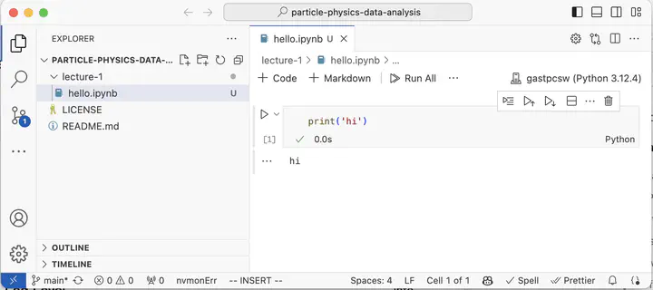
Start jupyter in VSCode
- Use your shell to create a folder
mkdir -p ~/work/physics/tutorial
-
Open
VSCodeand select from the menuFile -> Open Folder ..., then choose the folder you just created~/work/physics/tutorial.- Alternatively you can
cd ~/work/physics/tutorial code . -
Create a new file named
test.ipynb -
Now click on the right top and select the
pythonyou use forjupyter. It should be the one in thevenvearlier. -
Now type in one cell
print("hi")
- Press
CTRL+Enter, now you should run the cell and seehi.
Run iminuit tutorial
- iminuit is the
pythonversion of the famous Minuit software library. - Now you just copy and paste code on iminuit tutorial and test that you setup all softwares.
- Put this in one cell
# basic setup of the notebook
from matplotlib import pyplot as plt
import numpy as np

# everything in iminuit is done through the Minuit object, so we import it
from iminuit import Minuit

# we also need a cost function to fit and import the LeastSquares function
from iminuit.cost import LeastSquares

# display iminuit version
import iminuit
print("iminuit version:", iminuit.__version__)
# our line model, unicode parameter names are supported :)
def line(x, α, β):
    return α + x * β


# generate random toy data with random offsets in y
rng = np.random.default_rng(1)
data_x = np.linspace(0, 1, 10)
data_yerr = 0.1  # could also be an array
data_y = rng.normal(line(data_x, 1, 2), data_yerr)
least_squares = LeastSquares(data_x, data_y, data_yerr, line)

m = Minuit(least_squares, α=0, β=0)  # starting values for α and β

m.migrad()  # finds minimum of least_squares function
m.hesse()   # accurately computes uncertainties
- Press
CTRL + Enterand you should see the plots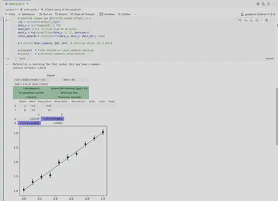
Screen shot of iminuit result
That’s it, and you’ve finished all tasks in this lecture. Congratulations!